PRACTICAL CASE STUDIES · LFS-1 · UPDATED 3 NOVEMBER 2026
Liquidity & Funding Simulator
Sell Investments or Borrow Against Them? Comparing Cash Buffers, Tax and Debt
A company needs £300,000 for equipment today. Should it sell investments, borrow against them, or combine both?
The company has £150,000 cash and a £1.5 million share portfolio. It wants to preserve a £100,000 cash reserve for operating needs. A separate £400,000 net receipt from the agreed sale of another asset is expected in month 12.
The payment and the expected receipt are the same under every plan. What changes is the cost, the investments retained and the resilience of the cash buffer.
The starting position
| Input | Assumption |
|---|---|
| Payment / available cash | £300,000 / £150,000 |
| Minimum cash reserve | £100,000 |
| Portfolio / tax cost basis | £1,500,000 / £900,000 |
| Receipt / analysis period | £400,000 in month 12 / 24 months |
| Loan / fees | 7% nominal annual interest, paid monthly / no fees |
| Eligible collateral value | 50% of the remaining portfolio |
| Other monthly cash flow / capital growth | £0 / 0% per year |
| Tax on positive realised gains | Illustrative 25%; no interest tax relief |
The 25% rate is an explicit case assumption, not a tax determination. Tax is set aside at sale and paid in month 9, an illustrative timing input. No dividends, cash interest or tax credits for losses are included.
1. Base case: the lower initial cost is not the whole result
Cash alone cannot fund the payment: it is £150,000 short at the start. LFS flags that plan as unfunded. The table compares the three initially funded alternatives. The combined plan raises £100,000 net from sales and borrows £200,000, with no opening cash contribution.
| Measure | Sell | Borrow | Combine |
|---|---|---|---|
| Gross investments sold | £333,333 | £0 | £111,111 |
| Tax on initial sale | £33,333 | £0 | £11,111 |
| Opening loan | £0 | £300,000 | £200,000 |
| Interest paid | £0 | £21,000 | £14,000 |
| Initial sale tax + interest | £33,333 | £21,000 | £25,111 |
| Lowest available cash | £150,000 | £130,750 | £137,167 |
| Cash at month 24 | £550,000 | £229,000 | £336,000 |
| Investments at month 24 | £1,166,667 | £1,500,000 | £1,388,889 |
| Debt at month 24 | £0 | £0 | £0 |
| Cash after hypothetical final sale | £1,600,000 | £1,579,000 | £1,586,000 |
First, read the funding. Raising £300,000 net requires a £333,333 sale. With proportional tax basis, 40% of the sale is gain; taxing that gain at 25% sets aside £33,333.
Then read the cost and reserve. Borrowing incurs £21,000 interest before repayment in month 12, £12,333 below the initial sale tax. But its minimum cash is £130,750 rather than £150,000. The combined plan sits between them.
Finally, compare a common endpoint. If all remaining shares are sold in month 24 at unchanged prices and the same tax rate, with all debts and modelled taxes settled, borrowing leaves £21,000 less cash than selling. The difference is paid interest: deferred tax is not tax permanently saved.
The final sale is a comparison convention, not a planned transaction. The acquired equipment is excluded equally from every plan. Amounts are rounded to the nearest pound.
2. What if the receipt arrives six months late?
Change only the receipt date from month 12 to month 18. The equipment payment remains due today and loan interest stays at 7%.
| Measure | Sell | Borrow | Combine |
|---|---|---|---|
| Tax + interest: base | £33,333 | £21,000 | £25,111 |
| Tax + interest: delayed receipt | £33,333 | £31,500 | £32,111 |
| Lowest cash: delayed receipt | £150,000 | £120,250 | £130,167 |
| Cash after hypothetical final sale | £1,600,000 | £1,568,500 | £1,579,000 |
The delay adds £10,500 to the full loan's cost and £7,000 to the combined plan. Selling creates no borrowing interest, so its cost is unchanged. Combined tax and interest now reach £32,111, close to the £33,333 initial sale tax, but that alone is not a complete economic comparison.
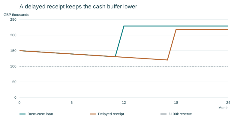
The reserve survives, with less room to spare. Minimum cash falls from £130,750 to £120,250, leaving £20,250 above reserve. This does not establish resilience to an indefinite delay or a cancelled receipt; another repayment source would need testing.
3. What if the delay coincides with market stress?
Keep the receipt in month 18. In month 6, impose a one-off 40% portfolio fall, increase loan interest to 9%, and reduce the eligible lending percentage from 50% to 35%. Prices then remain flat at their new level. These are imposed assumptions, not forecasts.
| Measure | Sell | Borrow | Combine |
|---|---|---|---|
| Tax + interest under stress | £33,333 | £38,000 | £36,444 |
| Lowest available cash | £150,000 | £114,250 | £126,167 |
| Collateral headroom in month 6 | No loan | £15,000 | £91,667 |
| Cash after hypothetical final sale | £1,250,000 | £1,112,000 | £1,158,000 |
The full loan is squeezed from two directions. Interest reaches £38,000 and minimum cash is £114,250, only £14,250 above reserve. The £900,000 portfolio supports £315,000 of debt under the entered rule, leaving only £15,000 above the £300,000 loan.
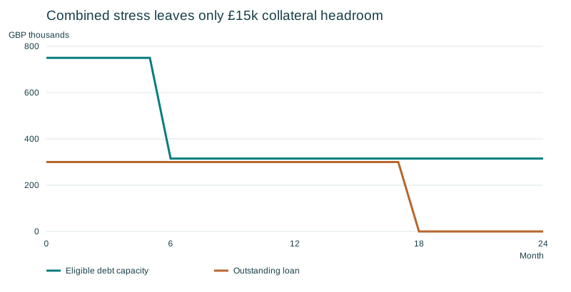
This scenario does not trigger a collateral repayment under the modelled rule. Headroom remains positive. The combined plan retains £91,667 of collateral headroom and a higher minimum cash balance. Selling retains less market exposure and therefore suffers less from the imposed fall. That does not mean the fall was predictable.
4. Make the choice against a cash constraint
| Priority | What this case shows |
|---|---|
| Retain investments and defer a sale | Borrowing adds interest, repayment obligations and collateral risk. |
| Preserve cash without a loan | Selling creates disposal tax and reduces retained market exposure. |
| Use a smaller loan while keeping some investments | The combined plan reduces interest and collateral pressure relative to full borrowing. |
| Preserve the minimum reserve | All three plans preserve it in these scenarios; full borrowing has the narrowest buffer under combined stress. |
The result is not “always borrow” or “always sell”. Compare funding, minimum cash and a common final position together. Here, the loan's lower initial cash cost comes with a tighter buffer and greater market exposure.
Repeat the analysis in LFS
Enter the starting figures and include the tax assumptions. Compare Base case, Receipt delayed and Combined stress. On a phone, choose two plans side by side. Expand the analysis and plan details when needed. Use Final position for the common-endpoint comparison and Cash flow & details to trace the monthly movements.
Open the worked example in Liquidity & Funding Simulator →
Method and boundaries
Recalculated with LFS 1.2.0 and checked against the live calculation file on 3 November 2026. Tables and charts use the same input set. Interest is paid before the receipt within each model month; month-end cash does not establish intramonth liquidity.
The case covers one entity, one currency and equal monthly periods. It excludes FX, dividends, cash yield, discounting and automatic refinancing. Tax basis is allocated proportionally, without tax-lot selection. National tax law, exemptions, losses and tax returns are not automatically calculated.
Collateral shortfalls are cured from available cash, even if that consumes the reserve. Forced sales are not simulated; an actual lender's contractual rights can differ. This is illustrative scenario analysis, not personalised lending, investment or tax advice.
Continue the LFS case-study series
LFS-1: compare selling, borrowing and a combined plan · Includes illustrative tax assumptions.
LFS-2: what happens when a collateral repayment is required? · Before tax.
LFS-3: can a partial sale protect the cash reserve? · Before tax.
LFS-4: can you meet the repayment demand when collateral falls and lending terms tighten? · Before tax.
These cases answer different questions. Their tax and stress assumptions differ; do not compare their figures as if the inputs were identical.