Practical Case Studies · DM-2
Debt Refinancing: How DM Finds a Lower Cost
Corporate Debt Lab’s algorithm, used in Debt Management and Lifecycle, identifies up to 24.14% lower aggregate conditional refinancing cost in a test of 1,000 synthetic portfolios. In each of the four tested scenarios, it costs less than all three benchmark strategies for at least 91.8% of the portfolios. Here is what lies behind those results.
The portfolios were created for DM’s research tests under a predefined protocol, covering different yield curves, one to five loans, and different maturities. We compare costs over 36 months, including fees. This is a modelled comparison at the decision date, not a historical Lifecycle backtest.
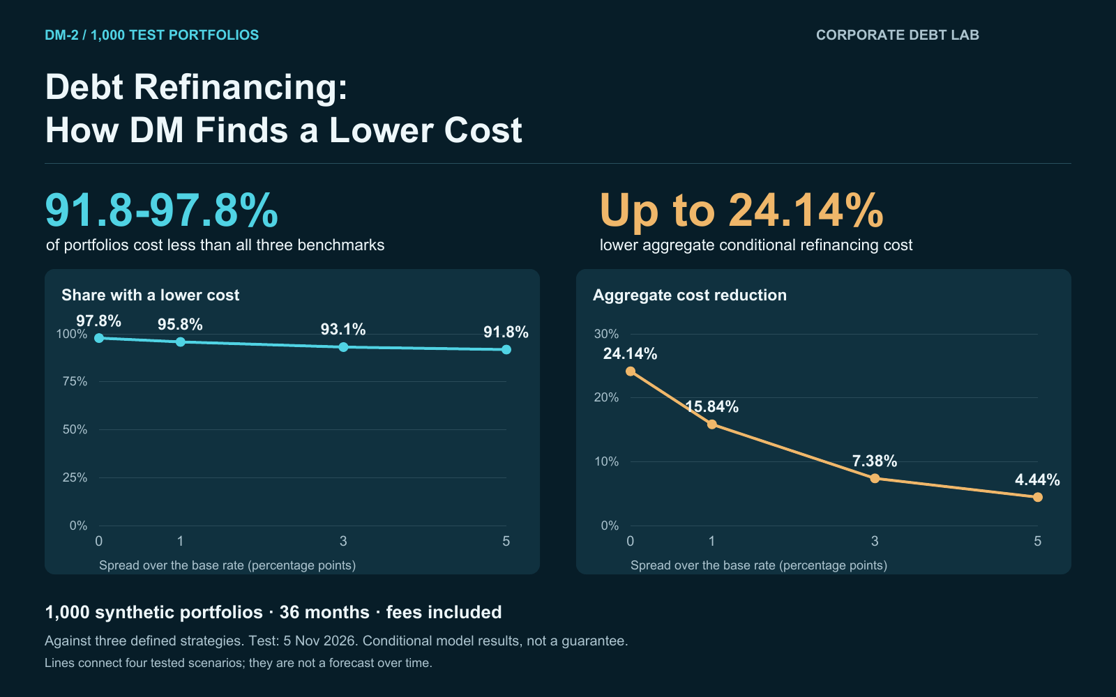
1,000 portfolios · 36 months · fees included · four funding-spread scenarios
The results at a glance
| Spread over the modelled base rate | Lower cost than all three benchmarks | Share of successful comparisons | Aggregate cost reduction |
|---|---|---|---|
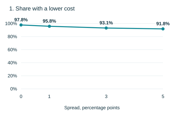
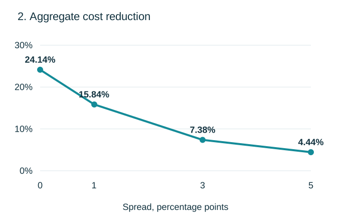
| 0 pp | 978 of 1,000 | 97.8% | 24.14% |
| 1 pp | 958 of 1,000 | 95.8% | 15.84% |
| 3 pp | 931 of 1,000 | 93.1% | 7.38% |
| 5 pp (severe stress) | 918 of 1,000 | 91.8% | 4.44% |
How to read the table: at a 1-percentage-point spread, DM costs less than each of the three alternatives in 958 cases. Aggregate cost across all 1,000 portfolios is 15.84% below the sum of the cheapest benchmark for each portfolio. The remaining cases are ties within the test tolerance.
What are we comparing DM against?
| Structure | Refinancing date | New loan term |
|---|---|---|
| 100% fixed | At maturity | 5 years |
| 70/30 fixed/floating | At maturity | 5 years |
| 100% fixed | 6 months before maturity | 7 years |
These are the benchmarks used in the 1,000-portfolio test. They differ from the historical Lifecycle set: 100% fixed, 100% floating and 70/30 fixed/floating. The percentages shown apply only to the benchmarks above.
What happens when funding becomes more expensive?
We use the same 1,000 portfolios in every scenario. We change the spread, not the sample. The spread is added to the modelled base rate; it is not the loan’s total interest rate.
Scenario 1: the spread increases to 3 percentage points
Compared with the zero-spread scenario, the share of successful comparisons falls from 97.8% to 93.1%, while aggregate cost reduction falls from 24.14% to 7.38%. The algorithm still frequently finds a cheaper option, but the size of the advantage narrows.
Scenario 2: the spread reaches 5 percentage points
Under this severe stress, DM remains cheaper than all three benchmarks in 918 of 1,000 cases. Aggregate cost is 4.44% lower. This marks the edge of the tested range; we do not claim that a 5-percentage-point spread is typical or rare for all companies.
The two measures answer different questions: how often DM finds an advantage and how large the aggregate financial effect is. For an individual client, DM compares their loan maturities, structures and refinancing dates. The decision should be based on available terms and the net benefit after fees.
Fees are 1% for new financing and 1% for early repayment, where applicable. All cases are included, including modelled negative costs.
Source: CDL, test recorded on 5 November 2026, SYNTHETIC_1000 / synthetic/results.jsonl; aggregation on 6 November 2026. Results refer to the tested version. The model was not rerun for this article.